Assignment 11 - Polar Equations
Faith Hoyt
In assignment 10 we investigated some parametric equations. Now, we want to take a look at polar equations. We are going to investigate our polar equation
![]()
In doing this we are not only going to look at the effect that a, b and k have on our graph, but we will also compare this to the equation ![]() , and replace our cosine function with a sine function.
, and replace our cosine function with a sine function.
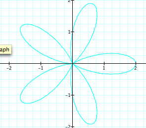
First, recall that when a and b are equal and k is an integer this will give us what is referred to as an "n-leaf rose." So, let's investigate this concept in the video below. We will set a = b = 1 and let k vary between 2 and 10 so we can see this affect.
Now, let's take this equation apart by looking at what each variable will affect. In this first case, I have fixed a and b and will vary k from 1 to 5.
![]()
![]()
![]()
![]()
![]()
All together:
Thus, from our graphs above, we can determine that our k value will affect the number of leaves that the graph has.
One more thing to look at when a = b. What happens if we make these values negative?
![]()
Notice, our graph is just rotated 180 degrees, or flipped across the y-axis. Now, let's compare two graphs: one where a = b = -1 and k = 5 and the other where a = b = 1 with k = 5.
![]()
![]()
We can see that the two graphs are the same thing, simply rotated by 90 degrees.
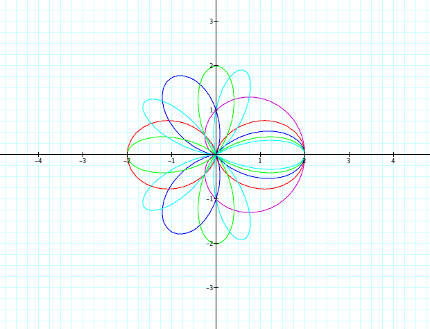
Now that we know what affect k has on our graphs, let's see what affect a and b have on our graphs. First we will see what happens when a < b. To do this we will fix our a and k values and allow b to vary.
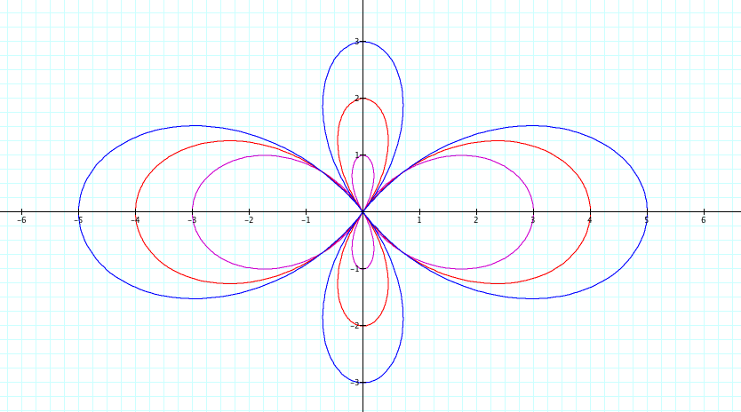
![]()
![]()
![]()
As we vary b to make it larger than a, notice that there is a smaller leaf that appears. Also, as we move from each graph we increase their intersection points by one. For example, the first graph intersects the x-axis at 3 and -3 while the red graph intersects the x-axis at 4 and -4.
Now, let's look to see what happens when a > b. To do this I will fix b and k and vary a.
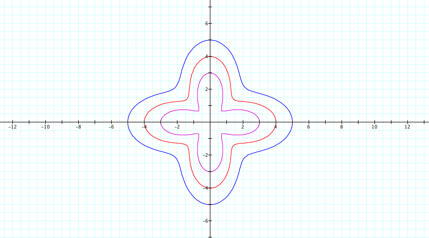
![]()
![]()
![]()
As we vary a and make it larger than b while keeping k constant, we can notice a few things. First of all the form of the curve changes. The leaves slowly loose form and get further from the origin. Above, we can see that as our a gets larger, it slowly stops looking like it has leaves and begins to look like a "blob."
Now, we want to compare this to ![]() .
.
Effectively here we are setting a equal to 0. We can see together what happens as we set b = 1 and vary k from 1 to 10 in the movie below.
Let's look at it in steps.
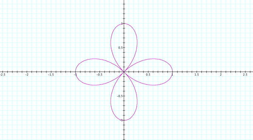
![]()
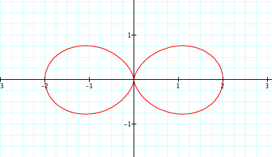
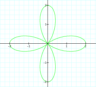
We can see that the intersections are at the points of the values of b. In other words, our b is equal to 1. Notice that our graph intersects the axes at x = -1, 0, 1 and at y = -1, 0, 1. Thus, the value of b determines where the intersection points will be and thus the largeness of the graph. Now, note that when we set our k = 2 yet there are 4 leaves. Interesting! Let's look at one more case to see what happens when k is odd.
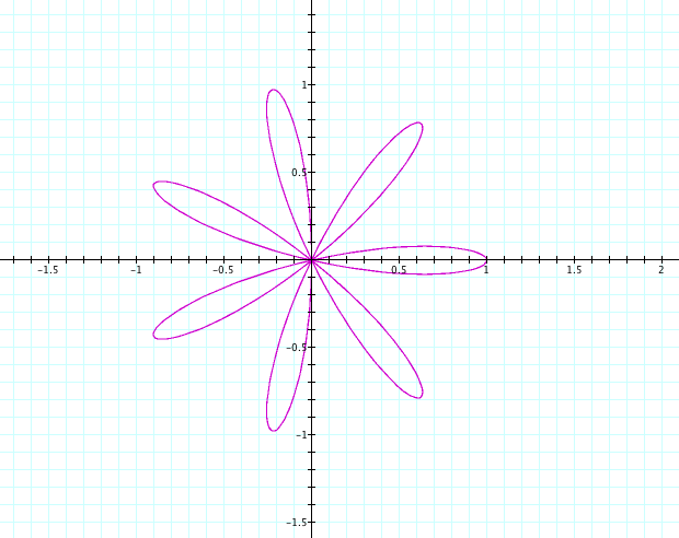
![]()
Now this changes where our intersection points are. We really only have one intersection point outside of our origin at x = 1, which aligns with our b value. However, for the other leaves, they don't intersect any where. We can see that all of our leaves are the same size. Thus if one of the leaves intersects at 1 we can say it has a length of 1 and then can generalize this to the rest of the leaves and say that they all have a length of 1. We noted above that when we set k =2 (which is even) there were 4 leaves. Now, we set k = 7 and we have 7 leaves.
We can now make a generalization! When our a value is 0, our k value will determine the number of leaves on the graph. When k is odd, there will be that number of leaves (i.e. when k = 7 there were 7 leaves). When k is even, there will be 2k number of leaves (i.e. when k = 2 there were 4 leaves or 2(2) leaves).
What happens when we replace our cosine function with sine to give us ![]() ?
?
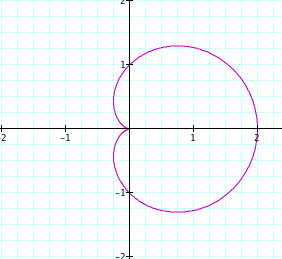
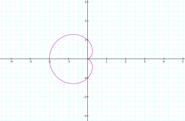
Let's first look at what it will look like when we compare it with our cosine function.
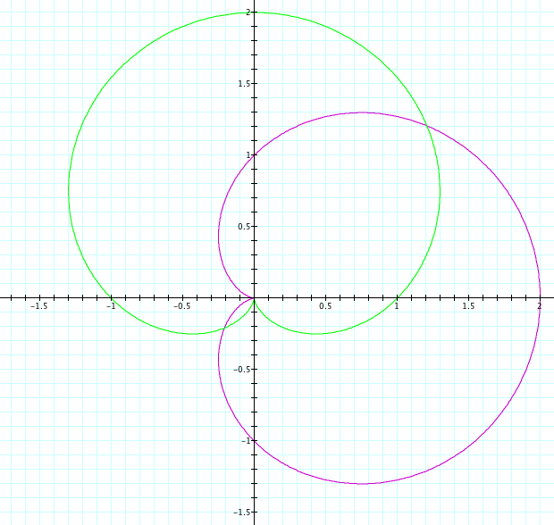
![]()
![]()
In this case a = b = k = 1. There are a few things we can notice. With our original graph (purple) our x-intercepts are at the origin and then at 2. The y-intercepts are at 0, -1 and 1. With our new sine graph (green) they are reversed. Our x-intercepts are at 0, -1 and 1 and our y-intercepts are at the origin and 2. If we think about the graphs of sine and cosine we can kind of see this and how it's almost like the sine graph is shifted from the cosine graph. Another thing to note is that it appears that the new graph is rotated 90 degrees about the origin. Is this going to be the case all the time? Let's check it out!
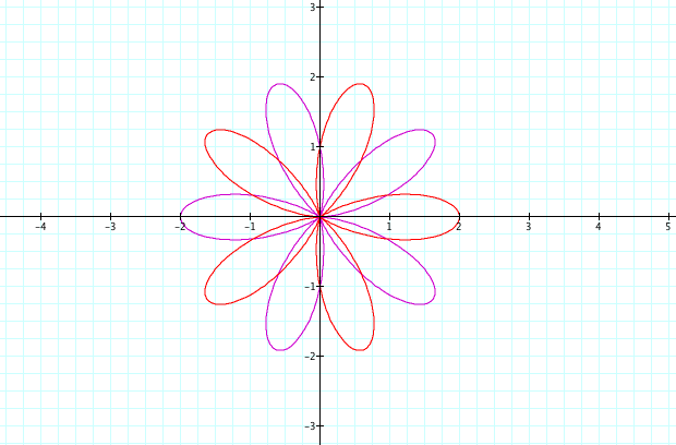
What if we let k = 2?
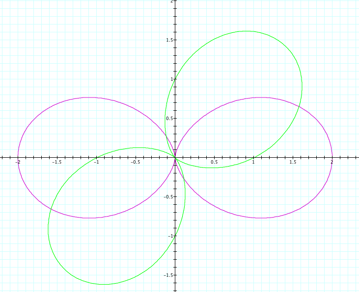
![]()
![]()
Once again this graph proves to be interesting. Since our k = 2 we have 2 leaves in both of our graphs. However, if our graph was rotated 90 degrees then it would appear to make up a shape that looked like a 4 leaf figure. So, visually we can see that the graph appears to be rotated at 45 degrees rather than 90 degrees. Note that this is 90 divided by 2 or 90 divided by k. This make sense. When k = 1 we would get 90/1 = 90 which was the degree it was rotated by. Now we have 90/2 = 45 which is the degree that it is rotated by. Do you think this will hold true? Let's look at one more case.
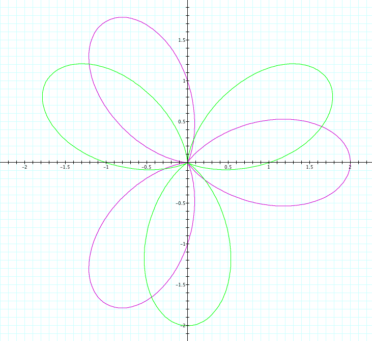
![]()
![]()
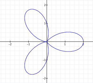
Going from our theory above, since k now is equal to 3, we should get a rotation of degree 90/3 = 30. Though we cannot measure this exactly, by looking at the graph it does in fact appear that it was rotated by 30 degrees. We also now have three leaves. This pattern, though it gets harder to discern, should keep up.
What happens when a<b?
Let's set a = 1, b = 2 and k = 3.
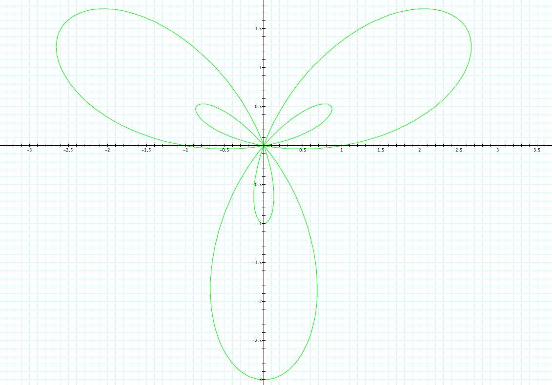
![]()
Notice that we still have k number of leaves and if we were to put our original cosine function on the same graph we could see that this is in fact rotated 30 degrees. There is one main difference to note though. There is a new set of leaves that is created! It appears that they are the smaller versions of the larger graph.
Here we can see how it would change if we fixed a and k and allowed b to vary:
As we can see, as b gets larger, the graph also gets larger and takes up more area. One interesting thing to note is as the graph gets closer to zero it starts to loose shape until it is a circle at b = 0. We can see this mathematically as this would simply give us an equation of r = 1 or a radius of 1.
What happens when a > b?
In order to look at this fully, we will fix our b and k values and vary our a value.
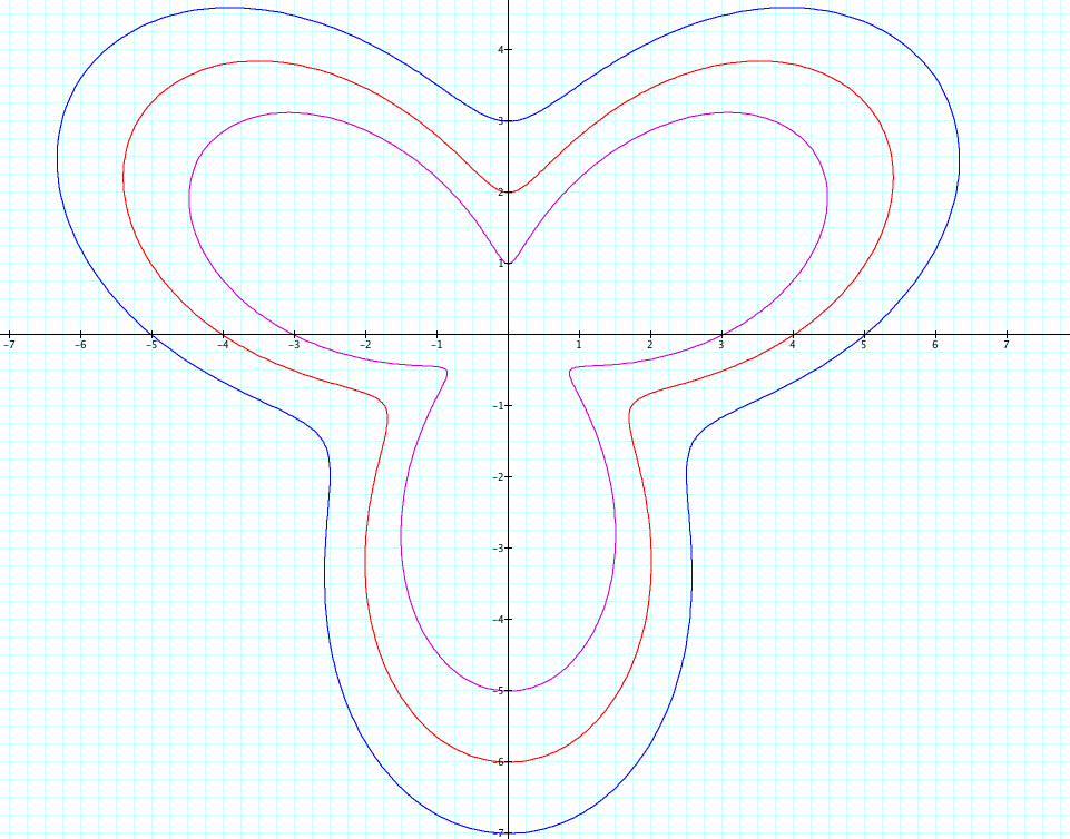
![]()
![]()
![]()
If we fix b at 2 and k at 3 but vary our a, as a gets larger the form of the curve begins to loose shape and starts to almost loosen. One could hypothesize that as a gets infinitely larger, the shape will eventually turn into a circle. Also, an important thing to recognize is the intercepts. For the x-intercepts, the graph crosses the x axis at the positive and negative values of a (i.e. when a=4 the x-intercepts are -4 and 4). For the y-intercepts it's a little more tricky. On the positive y axis the intercept is at the difference of our a and b values (i.e. in our first graph the positive y-intercept is 1 which is the same as a-b = 3-2 = 1). For the negative y axis the intercept is the negative sum of the two variables (i.e. in our second graph the negative y-intercept is - (a+b) = - (4 + 2) = -6).
Generalizations we can make about this graph: